SIMULATION OF A BROWNIAN MOTION

## import pandas as pd
import numpy as np
import pandas as pd
import matplotlib.pyplot as plt
from bokeh.plotting import figure, show, output_file, output_notebook
from bokeh.models import HoverTool

output_notebook() # plot

<!-- <div class="bk-root">
    <a href="https://bokeh.pydata.org" target="_blank" class="bk-logo bk-logo-small bk-logo-notebook"></a>
    <span id="1001">Loading BokehJS ...</span>
</div> -->

mu, sigma = 0, 1/252
N = 1000
variation = np.random.normal(mu, sigma, N)
bm = np.cumsum(variation)
random_x = np.linspace(0, 1, N)
hover = HoverTool(tooltips=[
    ("(x,y)", "($x, $y)"),
])
p = figure(plot_width=900, plot_height=400, title= "Brownian motion", tools=[hover])


p.line(random_x, bm)
show(p)

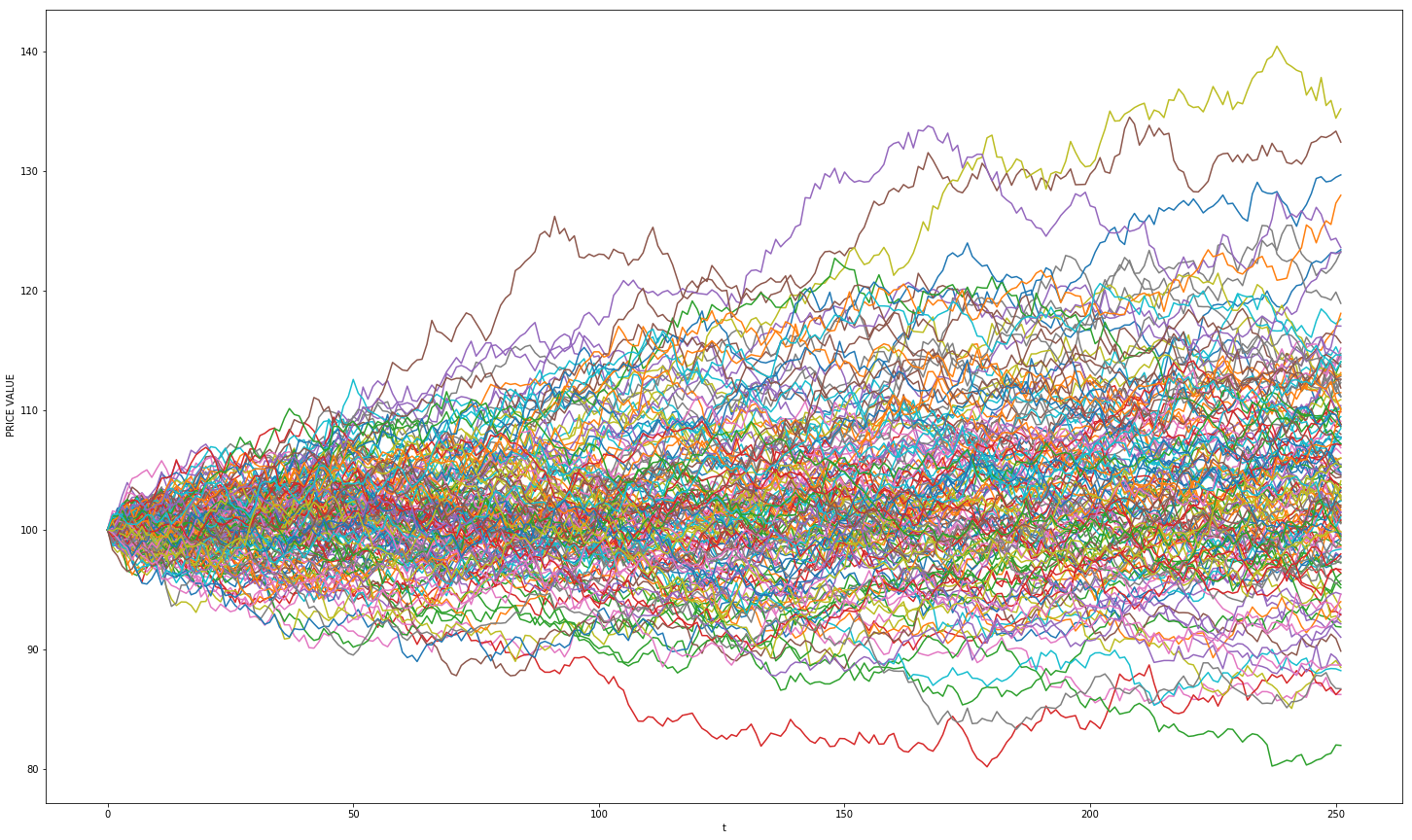
Asset price stochastic path

Suppose that the process followed by the underlying market variable is :

$dS = \mu Sdt + \sigma S dz$

where $dz$ is a Wiener process.

$S(t+\Delta t) = S(t) exp \left[ \left({\mu}-\frac{\sigma^2}{2} \right)\Delta t + \sigma \epsilon \sqrt{\Delta t} \right]$

#funtion of asset projection

def stockpaths(S, mu, sigma, T, n):
    mat=np.zeros((n, 252))
    for i in range(0,n):
        mat[i][0] = S
        for j in range(1,252):
            mat[i][j] = mat[i][j-1]*np.exp(((mu - 0.5*(sigma*sigma))*(T/252)) + (sigma*np.random.normal(0, 1, 1)*np.sqrt(T/252)))

    return mat

projections = stockpaths(S=100, mu=0.05, sigma=0.10, T=1, n=150)
#Plot graphics
# Ploting the default graphique
plt.figure(figsize=(25, 15))
plt.plot(pd.DataFrame(projections).transpose())
plt.xlabel('t')
plt.ylabel(' PRICE VALUE')
plt.show()

PRICES