Nielson Siegle and Nielson Siegle Svensson
NIELSON SIEGEL SVENSSON FOR INTERST RATE
This code is a litteral traduction in python of a part of the R code in the paper [1]
1.COMISEF WORKING PAPERS SERIES WPS-031 30/03/2010 “Calibrating the Nelson–Siegel–Svensson model” M. Gilli Stefan Große E. Schumann.
# -*- coding: utf-8 -*-
"""
Created on Mon Jul 03 09:32:36 2017

@author: gv4723
"""
from __future__ import division
import numpy as np
import pandas as pd
import matplotlib.pyplot as plt

# Nielson siegle svensson
# Calibration par Evolution Differentielle pour obtenir les beta de la fonction de lissage de Nielson siegel svensson
# Ce code est une tradution du code R de

# import pandas as pd

# NS simple

#def NS(betaV, mats):
#    gam = mats / betaV
#    y = betaV[1] + betaV[2] * ((1 - np.exp(-gam))/(gam)) + betaV[3] * (((1 - np.exp(-gam)) / (gam)) - np.exp(-gam))
#    return  y


# Equation du model de NSS version plus rapide
# nelson--siegel--svensson 2 (a bit faster)
# IN : solution betaV : mats : maturités
# OUT : les taux ou les données....

# Un warning est levé a ce niveau du fait que en python 2 la division par defaut du signe / est entiere...
def NSS2(betaV, mats):
    gam1 = mats / betaV[4]
    gam2 = mats / betaV[5]
    aux1  = 1 - np.exp(-gam1)
    aux2 = 1 - np.exp(-gam2)
    y = betaV[0] + betaV[1] * (aux1 / gam1) + betaV[2] * (aux1 / gam1 + aux1 - 1) + betaV[3] * (aux2 / gam2 + aux2 - 1)
    return (y)

# Fonction objective, la fonction à minimiser qui correspond à la distance entre les données et la fonction
# generic objective function
# In : Vecteur solution optimale betaV, data contient le modele à utiliser pour le calibrage, et les données sur lesquelles calibrer le modèle.
# Out : distance entre modèle et données réelles

def OF(betaV, data):

    mats =data.get("mats") # Les maturités
    yM = data.get("yM") # Les taux
    # model = data.get("model") # Le nom du modèle à utiliser, NS ou NSS2
    y = NSS2(betaV,mats)

    # crossprod() : Somme des carrées de ,
    # qui correspond donc à la distance entre le modèle y et les données yM
    # Pour changer la distance utilisé, c'est ici que ca se passe :
    aux=(y-yM)
    aux =  np.dot(aux,aux)
    return(aux)

#################### FONCTIONS CONCUES POUR ETRE UTILISE AVEC DES ARRAYS

# Fontions qui devront etre utilisées en DE
def mRU(m,n):
    return np.random.uniform(size=(m,n))

def mRN(m,n):
    return np.random.normal(size=(m,n))

def shift(x):
    rr = x.size
    return np.hstack((x[rr-1],np.array(x[range(rr-1)])))

def soustrac1(x, maxV):
    return x + maxV

def pen(mP, pso, vF):
    minV = pso.get("min")
    maxV = pso.get("max")
    ww = pso.get("ww")

    # max constraint: if larger than maxV, element in A is positiv
    # A = mP - (maxV)
    A = np.apply_along_axis(soustrac1,0,mP,maxV=-1*maxV)
    A = A + abs(A)

    # max constraint: if smaller than minV, element in B is positiv
    # B = minV - mP
    B = np.apply_along_axis(soustrac1,0,-1*mP,maxV=minV)
    B = B + abs(B)

    ## beta 1 + beta2 > 0
    C = ww * ((mP[0,:] + mP[1,:]) - abs(mP[0,:] + mP[1,:]))
    A = ww * np.sum((A + B),axis = 0) * vF - C
    return(A)

# DE stand for Differential Evolution
def DE(de,dataList,OF):

    # main algorithm
    # ------------------------------------------------------------------
    # set up initial population
    #mP = de.get("min") + np.dot(np.diag(de.get("max") - de.get("min")) , mRU(de.get("d"),de.get("nP")))
    mP = np.apply_along_axis(soustrac1, 0, np.dot(np.diag(de.get("max") - de.get("min")) , mRU(de.get("d"),de.get("nP"))) ,maxV = de.get("min"))

    # include extremes
    mP[:,0:de.get("d")] = np.diag(de.get("max"))
    mP[:,(de.get("d")):(2*de.get("d"))] = np.diag(de.get("min"))

    # evaluate initial population
    vF = np.apply_along_axis(OF, 0, mP,data = dataList)
    #vF = apply(mP,2,OF,data = dataList)

    # constraints
    vP = pen(mP,de,vF)
    vF = vF + vP

    # keep track of OF
    Fmat = np.empty((de.get("nG"), de.get("nP")), dtype=float)

    for g in range(de.get("nG")):
        # update population
        vI = np.random.choice(range(de.get("nP")), de.get("nP"))
        R1 = shift(vI)
        R2 = shift(R1)
        R3 = shift(R2)

        # prelim. update
        mPv = mP[:,R1] + de.get("F") * (mP[:,R2] - mP[:,R3])

        if de.get("R") > 0:
            mPv = mPv + de.get("R") * mRN(de.get("d"),de.get("nP"))

        #
        mI = mRU(de.get("d"),de.get("nP")) > de.get("CR")
        mPv[mI] = mP[mI]

        #
        vFv = np.apply_along_axis(OF, 0, mPv,data = dataList)

        # constraints
        vPv = pen(mPv,de,vF)
        vFv = vFv + vPv
        vFv[np.where(np.isinf(vFv))] = 1000000
        vFv[np.where(np.isnan(vFv))] = 1000000
        # find improvements
        logik = vFv < vF
        mP[:,logik] = mPv[:,logik]
        vF[logik] = vFv[logik]
        Fmat[g,:] = vF

    # g in 1:nG
    sGbest = np.min(vF)
    sgbest = np.argmin(vF)

    # return best solution
    return ({"beta" : mP[:,sgbest], "OFvalue" : sGbest, "popF" : vF, "Fmat" : Fmat})
# Import of the yiel curve data
df = pd.read_csv("yield_curve_spot_bce.csv", header=None, decimal=",")
print(df)
# application de l'evolution differentielle appliqué à Nelson siegel svennsson
# maturites
mats = df[0]

# taux
yM = df[1]

#
de = {"min"	: np.array([0.,-15,-30,-30,0  ,2.5]),# minimum du vecteur des paramètres à estimer
            "max"	: np.array([15, 30, 30, 30,2.5,5 ]),# Le maximum du vecteur des paramètres
		"d"	: 6, # Dimension du param-tre à estimer ou effectif de la population
		"nP"	: 200,
		"nG"	: 600,
		"ww"	: 0.1,
		"F"	: 0.50,
		"CR"	: 0.99,
		"R"	: 0.00 # random term (added to change)
}

dataList = {"yM" : yM, "mats" : mats, "model" : NSS2}
            0     1
0    0.333333 -0.88
1    0.166667 -0.87
2    0.111111 -0.87
3    1.000000 -0.87
4    2.000000 -0.86
5    3.000000 -0.78
6    4.000000 -0.64
7    5.000000 -0.47
8    6.000000 -0.28
9    7.000000 -0.10
10   8.000000  0.06
11   9.000000  0.21
12  10.000000  0.35
13  11.000000  0.46
14  12.000000  0.56
15  13.000000  0.65
16  14.000000  0.73
17  15.000000  0.79
18  16.000000  0.85
19  17.000000  0.91
20  18.000000  0.95
21  19.000000  1.00
22  20.000000  1.03
23  21.000000  1.07
24  22.000000  1.10
25  23.000000  1.13
26  24.000000  1.16
27  25.000000  1.18
28  26.000000  1.20
29  27.000000  1.22
30  28.000000  1.24
31  29.000000  1.26
32  30.000000  1.28
# Callibrage des beta par evolution différentielle
sols = DE(de = de,dataList = dataList,OF = OF)
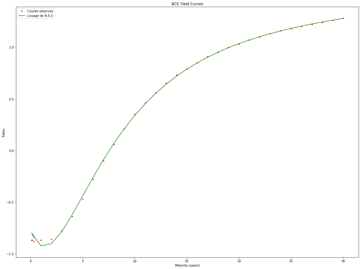
# Courbe des taux interpolée par NSS
courbe = NSS2(sols["beta"], mats)
plt.figure(figsize=(20, 15))
plt.plot(df[0], df[1] ,'r.',  label="Courbe observée")
plt.plot(df[0], courbe,'g',  label="Lissage de N.S.S.")
plt.legend() # Afficher la légende
plt.title('BCE Yield Curves')
plt.ylabel('Rates')
plt.xlabel('Maturity (years)')
Text(0.5, 0, 'Maturity (years)')
NIELSON SIEGEL FOR INTEREST RATE
This is a simple implementation of Nielson Siegel model for interest rate interpolation. Simple, because the calibration is made with the scipy optimize tool.
# -*- coding: utf-8 -*-
"""
Created on Sun Mar 5 13:41:37 2017
@author: workenv
"""
# CALIBRATION DU MODEL DE NIELSON SIEGEL
import pandas as pd
import numpy as np
import matplotlib.pyplot as plt
# import scipy as sc
from scipy.optimize import minimize, rosen, rosen_der
# df = pd.read_csv("yield_curve_spot_bce.csv", header=None, decimal=",")
to=df[0]
# Fonction d'optimisatiion,
# minimisation de la somme des écarts entre taux modélisés et taux théoriques
def fun(x,to):
return sum(((x[0]+x[1]*((1-np.exp(-to/x[4]))/(to/x[4]))+x[2]*(((1-np.exp(-to/x[4]))/(to/x[4]))-np.exp(-to/x[4]))+x[3]*(((1-np.exp(-to/x[5]))/(to/x[5]))-np.exp(-to/x[5])))-df[1])**2)
# Optimisation sans contraintes, méthode du simplexe
# res_sc = minimize(fun, (.1,1,1,1,1,1),args=(to), method= "Nelder-Mead")
# optimisation sous contraintes
cons = ({'type': 'ineq', 'fun': lambda x: x[1] + x[2]})
bnds = ((0, None), (None, None),(None, None), (None, None),(0, None), (0, None))
res_c = minimize(fun, (0.1,1,1,1,1,1),args=(to), method= "SLSQP",bounds=bnds)
#Fonction de calcul des courbes modélisées
# ycm = yields curves estimated
def ycm(to, x):
return x[0]+x[1]*((1-np.exp(-to/x[4]))/(to/x[4]))+x[2]*(((1-np.exp(-to/x[4]))/(to/x[4]))-np.exp(-to/x[4]))+x[3]*(((1-np.exp(-to/x[5]))/(to/x[5]))-np.exp(-to/x[5]))
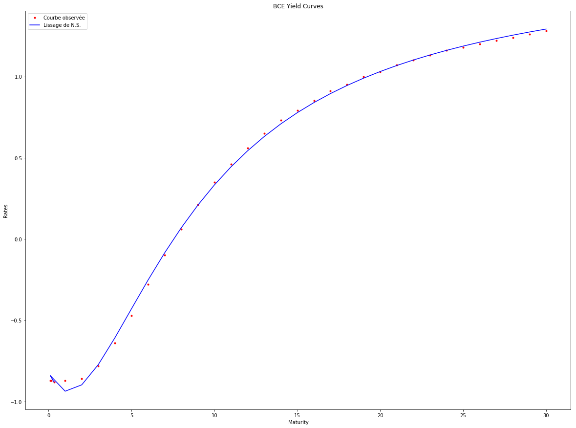
#Graphiques de comparaison entre courbe observée et courbe modélisée
plt.figure(figsize=(20, 15))
plt.plot(df[0], df[1] ,'r.', label="Courbe observée")
plt.plot(df[0], ycm(to,res_c.x),'b', label="Lissage de N.S.")
plt.legend() # Afficher la légende
plt.title('BCE Yield Curves')
plt.ylabel('Rates')
plt.xlabel('Maturity')
#f2 = sc.interpolate.interp1d(df[0], df[1], kind='cubic')
#plt.plot(df[0], df[1] ,'o-', df[0], f2(df[0]),'g-')
#
#tck = sc.interpolate.splrep(df[0], df[1], s=0)
Text(0.5, 0, 'Maturity')
Who is better: NIELSON SIEGEL SVENSSON with DE vs NIELSON SIEGEL with simplex
plt.figure(figsize=(20, 15))
plt.plot(df[0], df[1] ,'r.',  label="Courbe observée")
plt.plot(df[0], ycm(to,res_c.x),'y',  label="Lissage de N.S.")
plt.plot(df[0], courbe,'g',  label="Lissage de N.S.S.")
plt.legend() # Afficher la légende
plt.title('BCE Yield Curves')
plt.ylabel('Rates')
plt.xlabel('Maturity')
Text(0.5, 0, 'Maturity')
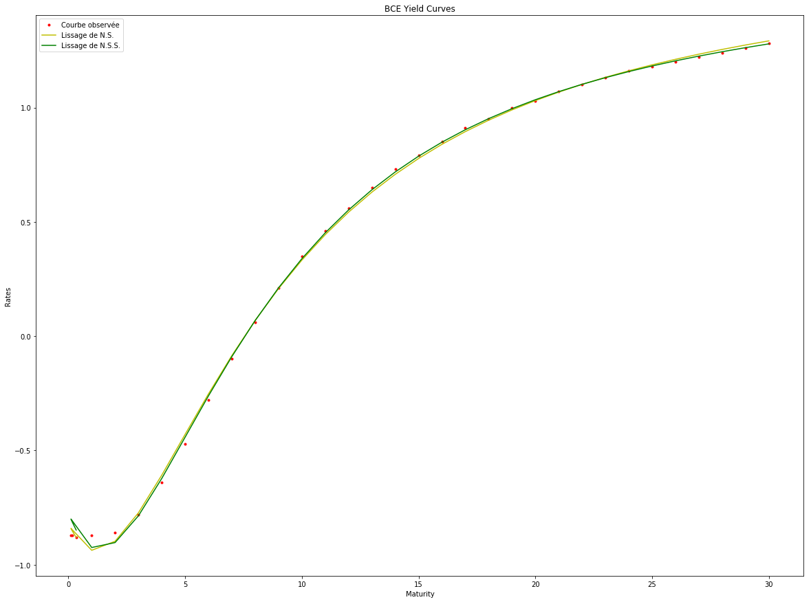
Nielson Siegel Svensson with calibration by Differential evolution seems to be better.